
With increased computing power comes increased access to large amounts of freely accessible data. People are tracking their lives with productivity, calorie, fitness and sleep trackers. Governments are publishing survey data left and right, and companies conduct audience testing that needs analyzing. There’s a lot of data out there even now, ready to be grabbed and looked at.

In this tutorial, we’ll look at the basics of the R programming language — a language built solely for statistical computing. I won’t bore you with Wikipedia definitions. Instead, let’s dive right into it. In this introduction, we’ll cover the installation of the default IDE and language, and its data types.
Installing
Table of Contents
R is both a programming language and a software environment, which means it’s fully self-contained. There are two steps to getting it installed:
- download and install the latest R: www.r-project.org
- download and install RStudio, the R IDE: www.rstudio.com
Both are free, both open source. R will be installed as the underlying engine that powers RStudio’s computations, while RStudio will provide sample data, command autocompletion, help files, and an effective interface for getting things done quickly. You could write R code in simple text files as in most other languages, but that’s really not recommended given how many commands there are and how complex things can quickly get.
After you’ve installed the tools, launch R Studio.
IDE Areas
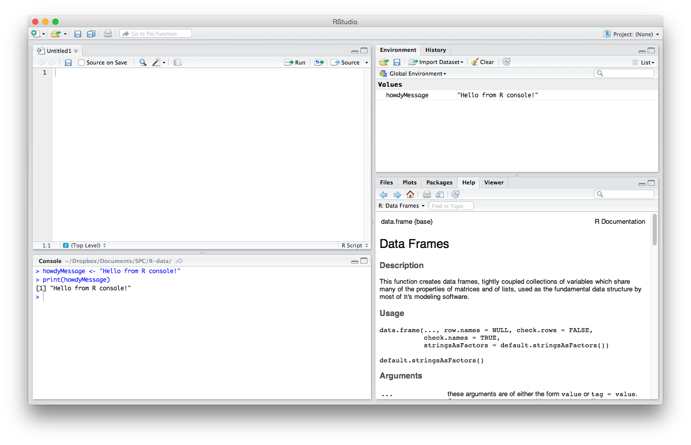
Let’s briefly explain the GUI. There are four main parts. I’ll explain the default order, though note that this can be changed in Settings/Preferences > Pane Layout.
The Editor
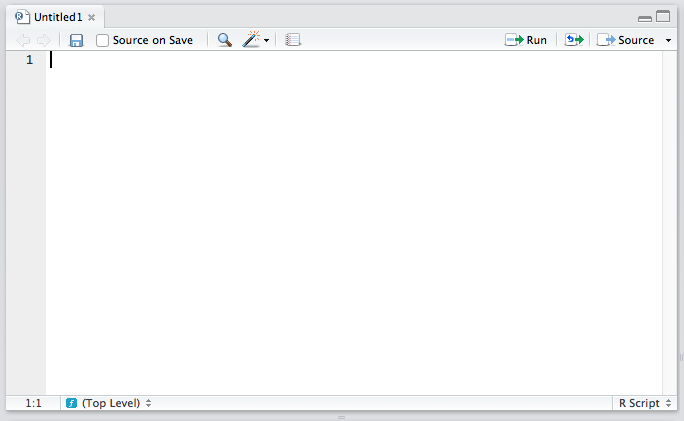
The top left quadrant is the editor. It’s where you write R code you want to keep for later — functions, classes, packages, etc. This is, for all intents and purposes, identical to every other code editor’s main window. Apart from some self-explanatory buttons, and others that needn’t concern you at this starting point, there’s also a “Source on Save” checkbox. This means “Load the contents of the file into my console’s runtime every time I save the file”. You should have this on at all times, as it makes your development flow faster by one click.
The Console
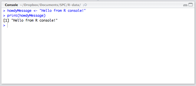
The lower left quadrant is the console. It’s a REPL for R in which you can test out your ideas, datasets, filters, and functions. This is where you’ll be spending most of your time in the beginning. Here’s where you verify that an idea you had works before copying it over into the editor above. This is also the environment into which your R files will be sourced on save (see above), so whenever you develop a new function in an R file above, it automatically becomes available in this REPL. We’ll be spending a lot of time in the REPL in the remainder of this tutorial.
History / Environment
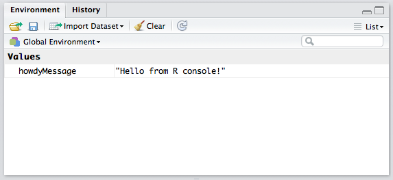
The top right quadrant has two tabs: Environment and History.
Environment refers to the console environment (see above) and will list, in detail, every single symbol you defined in the console (whether via sourcing or directly). That is, if you have a function available in the REPL, it will be listed in the environment. If you have a variable, or a dataset, it will be listed there. This is where you can also import custom datasets manually and make them instantly available in the console, if you don’t feel like typing out the commands to do so. You can also inspect the environment of other packages you installed and loaded. (More on packages at a later time.) Go ahead and play around with it; you can’t break anything.
History lists every single console command you executed since the last project started. It’s saved into a hidden .Rhistory file in your project’s folder. If you don’t choose to save your environment after a session, the history won’t be saved.
Misc
The bottom right panel is the misc panel, and contains five separate tabs. The first one, Files, is self-explanatory.
The Plots tab will contain the graphs you generated with R. It’s here that you can zoom, export, configure and inspect your charts and plots.
The Packages tab lets you install additional packages into R. A brief description is next to each available package, though there are many more than those listed there. We’ll go through package repositories in a later post.
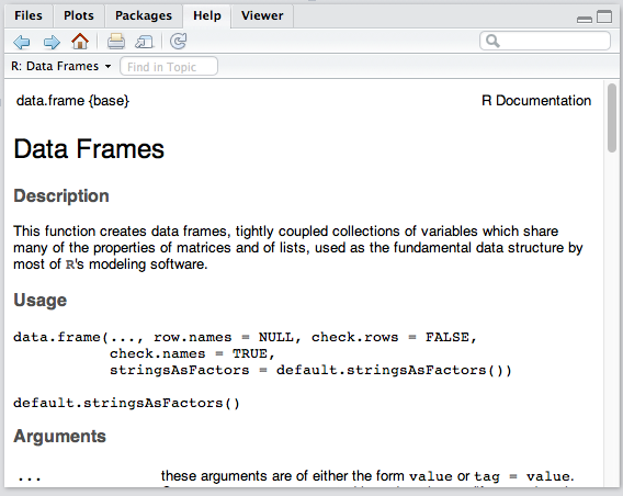
The Help tab lets you search the incredibly extensive help directory and will automatically open whenever you call help on a command in the console. (Help is called by prepending a command name with a question mark, like so: ?data.frame.)
Finally, the Viewer is essentially RStudio’s built-in browser. Yes, you can develop web apps with R and even launch locally hosted web apps within it.
Built-in datasets
In the text below, whenever I mention using a command, assume this means punching it into the console. So, if I say “We look at the help for DataFrames with ?data.frame”, you do this:
RStudio comes with some datasets for new users to play around with. To use a built-in dataset, we load it with the data function, and supply an argument corresponding to the set we want. To see all the available built-in sets, punch in data(), without an argument.
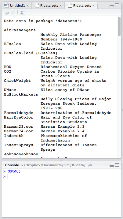
Looking at the list of available datasets, let’s load a very small one for starters:
data('women') You should see the women variable appear in the Environment panel, though its second field says <Promise>. A promise in this case merely means “The data will be there when you actually need it”. We told R to load this set, but we haven’t actually used it anywhere, so it didn’t feel the need to load it fully into memory. Let’s tell R we need it. In the console, print out the entire set by simply calling this:
women This is equivalent to:
print(women) Note: we’ll be using the former approach, simply because it’s less typing. Remember: in R, the last value that’s typed out without being an expression (like assigning or summing something) is what gets auto-printed to the console.
The numbers will be produced in the console, and the Environment entry for women should change. You should be able to see the data in the environment panel now, too, by clicking the blue expand arrow next to the variable name.
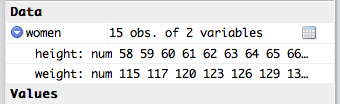
This set only has 15 entries, and as such offers nothing of value, but it’s good enough for playing around in.
To further study the set you’re dealing with, there are several functions to keep in mind (a demonstration of each can be seen below explanations):
nrow/ncolwill list the number of rows/columns respectively.summarywill output a summary about the set’s columns. In the case of thewomenset, we have two numeric columns (both columns are numeric, or in other words, each column is a numeric vector; more on data types and vectors later). And R knows that, when you ask it for an analysis of a numeric vector, it should give you the typical values for such collections: the minimum value in the set, the mean (average) between the minimum and the mean, the mean (average of all values), the mean between the mean and the maximum, and the maximum, the largest number in the column. It does this for both height and width. For different types of vectors (like ones where every element is a word instead of a number) the output is different.stris a different kind of summary. In fact,strstands for “structure” and it outputs a summary of a dataset’s structure. In our case, it will tell us that it’s a “data.frame” (a special data type we’ll explain later) with 15 obs (observations or rows) and two variables (or columns). It then proceeds to list all the columns in the DataFrame with some (but not all) of their values, just so we get a grasp on the kind of values we’re dealing with.dimgives you the dimensions of a dataset. Callingdim(women)gives us15 2, which means 15 rows and two columns.lengthcan be used to count the number of vertical elements in a set. In vectors (see below), this is the number of elements; in data sets likewomen, this is the number of columns:
> nrow(women) [1] 15 > ncol(women) [1] 2 > summary(women) height weight Min. :58.0 Min. :115.0 1st Qu.:61.5 1st Qu.:124.5 Median :65.0 Median :135.0 Mean :65.0 Mean :136.7 3rd Qu.:68.5 3rd Qu.:148.0 Max. :72.0 Max. :164.0 > str(women) 'data.frame': 15 obs. of 2 variables: $ height: num 58 59 60 61 62 63 64 65 66 67 ... $ weight: num 115 117 120 123 126 129 132 135 139 142 ... > dim(women) [1] 15 2 You’ll be using these functions a lot, so I recommend you get familiar with them. Load some of the other datasets and inspect them like this. There’s no need to know them by heart. This tutorial and the help files will always be around for reference, but it’s nice to be fluent in them anyway.
Data Types
R has some typical atomic data types you already know about from other languages, but it also provides some more statistics-inclined ones. Let’s briefly go through them. While explaining these types, I’ll talk about assigning them. Assigning in R is done with the “left arrow” operator or <-, as in:
myString <- 'Hello, World!' R is, however, very forgiving and will let you use the = assignment operator in top level environments like the console, if you don’t feel like typing out the arrow every time:
myString = 'Hello World' I suggest you get used to the arrow, though, as you won’t get very far without it.
To check the type (or class) of a variable, the class function can be used (though str from above does almost the same thing): class(myString).
Atomics
Atomic classes are basic types from which others are constructed.
Character
The character class is your typical string, a set of one or more letters:
> myString <- 'Hello World' > class(myString) [1] 'character' The [1] will be explained below, in the “Vectors” section.
Numeric
The numeric class corresponds to float in other languages. It indicates numeric values like 10, 15.6, -48792.5498982749879 and so on:
> myNum <- 5.983904798274987298 > class(myNum) [1] 'numeric' You can coerce (change type of) numeric string values into numeric types, like so:
> myString <- '5.60' > class(myString) [1] 'character' > myNumber <- as.numeric(myString) > myNumber [1] 5.6 > class(myNumber) [1] 'numeric' There’s also a special number Inf which represents infinity. It can be used in calculations:
> 1/0 [1] Inf Another “number” is NaN, which stands for “Not a Number”. This is what you get when you do something like 0/0.
Integer
Integers are whole numbers, though they get autocoerced (changed) into numerics when saved into variables:
> myInt <- 209173987 > class(myInt) [1] 'numeric' To actually force them to be integers, we need to invoke a function that manually coerces them, called as.integer:
> myInt <- as.integer(myInt) > class(myInt) [1] 'integer' You can prevent autocoercion by setting integers with an L suffix:
> myInt = 5L > class(myInt) [1] 'integer' Note that, if you give R a number that’s greater than what its memory can store, it autocoerces it into a real number, even if you put L at the end:
> myInt <- 2479827498237498723498729384 > class(myInt) [1] 'numeric' > myInt [1] 2.479827e+27 But if you then try to coerce that number into an integer, R will discard it because it simply can’t make integers that big. Instead of a number, you get “NA”, which is a special type in R indicating “Not Available”, also known as a missing value:
> myIntCoerced <- as.integer(myInt) Warning message: NAs introduced by coercion > myIntCoerced [1] NA > class(myIntCoerced) [1] 'integer' The NA is still a type of “integer”, but one without value.
Note that, when coercing numerics into integers, decimal places get lost. The same applies to coercing from numeric decimal strings:
> myString <- '5.60' > myNumeric <- 5.6 > myInteger1 <- as.integer(myString) > myInteger2 <- as.integer(myNumeric) > myInteger1 == myInteger2 [1] TRUE > myInteger1 [1] 5 Continue reading Introduction to R and RStudio on SitePoint.